Image Classification On CIFAR 10: A Complete Guide
Chapter I: Multiclass Logistic Regression
Picking up a worn mechanical pencil from the floor, a half-used Staedtler eraser, a metal 6-inch ruler, a notebook from Japan, and my computer, at 1am on a school night, October 3rd, 2020, I began to teach myself calculus.
Okay, not teaching myself. There’s no such thing as teaching yourself, these days, with the plethora of content out there. Opening the first lesson in Khan Academy’s Calculus AB playlist, I learned about limits.

Then derivatives. Then calculating them. Then linear algebra. Then multivariable calculus.
All I can say how grateful and fortunate I was to have had the opportunity to spend an upwards of 5 hours a day learning mathematics. I’m incredibly privileged in that respect— to have the time to engage in the beautiful ivory-tower-esque discipline, and to be able to now view machine learning and mathematics in a depth I would have not been able to attain before. So thank you, so, very much, everyone who accommodated, tolerated and communicated with me during that period.
Enter early November. Feeling satisfied with the breadth of mathematics I covered, I began coding in PyTorch. My first project was a simple univariate linear regression problem. With that under my belt, I approached something tougher, with the help of a tutorial.
Image classification with logistic regression.
contents
It’s a rather large tutorial, so I’ll put links here if you’d like to skip:
- The CIFAR-10 Dataset
- Data Wrangling
- Indexing into Data
- Using matplotlib to Display Images
- Transforming Images into Tensors
- Training and Validation Sets
- Batch Loading for Mini-Batch Gradient Descent
- The Hypothesis
- The Softmax Function
- Evaluation and Accuracy
- Cross-Entropy Cost Function
- Mini-Batch Gradient Descent
- Computing Gradient for a Single Batch
- Evaluating Cost and Accuracy on Validation Set
- Fitting the Model
- Is Low Accuracy Unavoidable with Logistic Regression?
- Google Colab Document
- Update rule for weights
a few disclaimers
I’ll be going through [most] of the code I used, but I’ll be putting more of an emphasis on the mathematics and inner working the code represents. Most of the code was snatched from Aakash’s fantastic tutorial on PyTorch from freeCodeCamp.org, but slightly changed to accommodate a slightly more complicated dataset (CIFAR instead of MNIST). I’ll include my full adapted code in the form of a Google Colab document at the end of this article.
This tutorial assumes a pretty solid understanding of many machine learning concepts, such as gradient descent, cost functions, linear regression, hyperparameters, and common notation, as well as mathematical concepts like matrix multiplication and partial derivatives.
notation
I generally use standard notation here.
- m is the length of the training set.
- features are the different inputs into an algorithm.
- subscripts generally represent libraries, and if you see a subscript like 23 it means the 3rd feature on the 2nd class.
- superscripts generally represent training examples
- j as a variable is usually used as a subscript to signify looping.
- I tend to say thetas interchangeably with “weights and biases”, since theta is often used instead of W or b in weights or biases.
- Throughout the tutorial, I sometimes switch between using column (e.g 10, 1) and row vectors (e.g 1, 10), but they mean the same thing.
- Whenever you see log(), think of it as ln().
# necessary librariesimport torch
import pandas as pd
import matplotlib.pyplot as plt
import numpy as np
One frog, two frog: The CIFAR-10 Dataset
CIFAR-10, a subset of the now defunct 80 Million Tiny Images Dataset was one of the many possible datasets that was easily accessible within the framework of the PyTorch library (coming ‘plug-and-play’ in the .datasets module). I wish I could say there was a more romantic story behind it, but I chose CIFAR-10 rather arbitrarily.
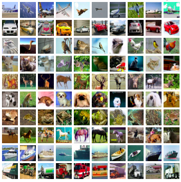
I decided to use logistic regression to create a model that would attempt to predict which of the 10 classes some image from this dataset would be predicted as.
Made up of 60,000 (50,000 for training/validation and 10,000 for test) 32x32 pixel images, CIFAR-10 has been an extraordinary resource for testing the accuracy of a variety of cutting-edge machine learning algorithms, as well as being a fantastic playground for machine learning experimentation.
Now, we load the dataset.
Loading, wrangling, & splitting — data preparation
It’s an incredible convenience to be able to download the data directly from the PyTorch library, instead of the CIFAR-10 site. De-pickling files was a bit intimidating.
>> import torchvision# import the training set (first 50,000 imgs) by setting train=True.>> trainset = torchvision.datasets.CIFAR10(root='./data', train=True,download=True)# import the test set (10,000 imgs) by setting train=False>> testset = torchvision.datasets.CIFAR10(root='./data', train=False, download=True)# define the ten labels manually.>> classes = ('plane', 'car', 'bird', 'cat', 'deer', 'dog', 'frog', 'horse', 'ship', 'truck')
Not much to explain mathematically or theoretically here. By accessing torchvision.datasets, we can access our CIFAR dataset.
indexing into data
Let’s access the first image in our dataset.
>> trainset[0]
(<PIL.Image.Image image mode=RGB size=32x32 at 0x7FF6E08F5908>, 6)
Indexing into trainset with typical notation returns two values. First, an intimidating string of letters and numbers, and 6. The fact that we are returned two values can create the correct image of trainset being a 50000x2 matrix, each example being a pair of image and correct answer, x and y.
That intimidating first value is a PIL.image object — a special code for that image, encoded and saved using the Python Pillow library.
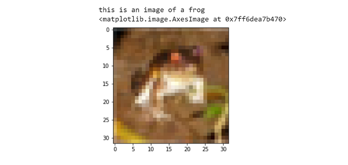
The comparatively simple second term is the ‘right answer’ for that image, the label. Glancing at our predefined label array, we can see that 6 represents an image of a frog. But how do we view our little frog friend?
using matplotlib to view images from dataset
We can use the standard matplotlib.pyplot library to plot our images as colored pixel values.
# you might have to use this magic function depending on your IDE
>> %matplotlib inline
The above code is a magic function. Depending on your IDE, this code will prevent graphs created by matplotlib to open in a different window (a popup) and will instead show them inline, underneath the code.
Now, we can plot our image.
>> example = 0# index into the 50,000 x 2 trainset vector, and store the label in the variable 'label'. Store the PIL object in variable 'image'.>> image, label = trainset[example] # print the label for the image by indexing label into classes.>> print("this is an image of a " + classes[label]# use imshow to show the PIL object image>> plt.imshow(image)
The image shown by this will show example -th training example from the training set. Executing this code will show us our first image from the training set, a frog, paired with it’s label.
Transforming images into matrices of numbers (tensors)
There isn’t a way for an algorithm to truly see an image. That’s why we need to find a way to represent an image with numbers, and individually feed each one of those numbers in to our algorithm as a feature.
To understand how we do this, we must take a brief look at simple color theory. More specifically, the Red-Green-Blue (RGB) model.
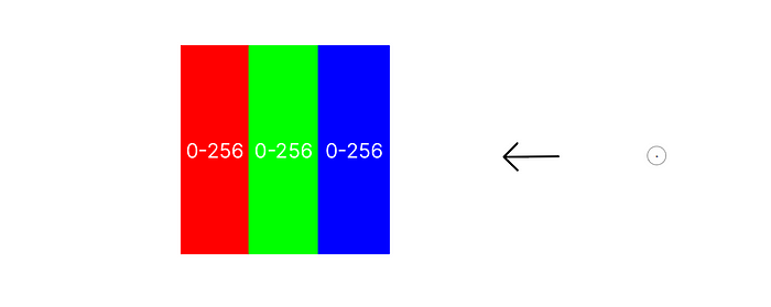
Every pixel on your screen, and every pixel in an image, is represented by three bars of primary red, green and blue. Each of these bars can be dialed up or down in intensity from 0–256 (why 256? think binary). Combinations of these three colors, each at some intensity between 0 and 256, creates every color we know. Large blocks of color are made up of many pixels with the same RGB values. One pixel’s color can be described by just three numbers.
Sensibly, then, we can represent a whole picture by defining it using it’s R, G, and B values for each pixel.
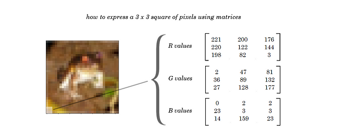
Formally, we can describe an image using 3 matrices that hold the individual R, G, and B color channels of each pixel. Each of the three matrices will be the same dimensions, the height x width of the image in pixels.
Thus, we can describe each image in our training set using a 3, 32, 32 matrix of pixel intensity values from 0–256. This gives us 3072 (3x32x32) features to plug into our dataset, if we unroll the image matrices into one long vector.
This is how an image sees. When an algorithm tries to predict the content of an image, it isn’t looking the way humans tend to recall and identify the things we see. When an algorithm predicts the content of an image, it’s really just comparing the number matrices with past number matrices and seeing which examples match up best.
Now we can confidently implement (the now trivial-seeming) code to do this image-to-matrix conversion.
>> import torchvision.transforms as transforms# directly access the training set again from .datasets, and set the transform keyword argument to transforms.ToTensor())>> datasetT = torchvision.datasets.CIFAR10(root='./data', train=True, download=True, transform=transforms.ToTensor())
At this stage, it’s most practical to think of tensors as any numerical object that can be operated on mathematically within a machine learning algorithm. Images are not tensors. Matrices, on the other hand, are.
Indexing into our new, transformed training set, we see that the first value on each row (training example) is no longer a PIL.image object, but a tensor, and more specifically, a matrix of dimensions 3, 32, 32. This makes the dimensions of our total training set [50000, 3, 32, 32].
>> example = imgTensor, label = datasetT[example]
>> print("size of image matrix: " + str(imgTensor.shape))
>> print("this is an image of a "+ classes[label]size of image matrix: torch.Size([3, 32, 32])
this is an image of a frog
We can still view the image using matplotlib.imshow even if it’s now in tensor format, requiring no change in syntax. As an added bonus, we can now index into custom values for the first dimension (x, 32, 32) to see the different color channels of the image individually (or :, all, to see the image normally)
# change the 0 (R) to 1 (G) or 2 (B) for different color channels. Additionally, recall that imgTensor represents just our first example.plt.imshow(imgTensor[0, 0:32, 0:32])
print("R channel of image 0 in dataset")
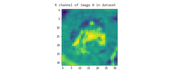
Note that Python defaults to showing graphs in a green colormap. Remember, when we use matplotlib to plot images, we’re treating the images as a heatmap of colored points that form an image. If you want actual red channel values, pass in the tensor to .imshow and use
>> plt.imshow(imgTensor[0, 0:32, 0:32], cmap='Reds')       # R
>> plt.imshow(imgTensor[1, 0:32, 0:32], cmap='Greens')     # G
>> plt.imshow(imgTensor[2, 0:32, 0:32], cmap='Blues')      # B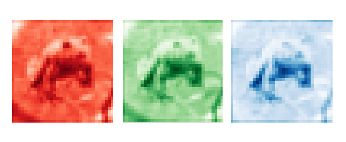
training and validation sets
I assume that if you’re reading this article, you have a solid understanding about the significance for splitting your initial X set into training and validation sets. In essence:
- the training set is used to train the parameters of a given model, and usually takes up around 60% of a total dataset.
- the cross-validation set is used to evaluate the model during training (e.g, to see if gradient descent is working properly), to diagnose over and underfitting, and to adjust hyperparameters like the learning rate. It usually takes up around 20% of the total dataset.
- the test set is used to report the accuracy of the completed model. It usually takes up around 20% of the total dataset.
Since PyTorch already loads the test set independently, let’s split our training set into a 80/20 ratio between training and cross-validation (CV) respectively. There are functions to do this that are built-in to PyTorch, but let’s create a function to shuffle the indexes of the training set and to split the set into whatever ratio we want, from scratch.
#length of training examples matrix (how many training ex.)(m).>> m = 50000# percentage of training set dedicated to CV.>> pCV = 0.2# give the amount of cross-validation examples from m.>> mCV = int(m*pCV)# print the lengths>> print("amount of training examples: " + str(m - mCV))
>> print("amount of cross validation examples: " + str(mCV))amount of training examples: 40000
amount of cross validation examples: 10000
Now, we can define a function that will shuffle the indices of our original training set and allow us to split it up into the amounts described above.
>> def splitIndices(m, pCV):     >> """ randomly shuffle a training set's indices, then split
    indices into training and cross validation sets. Pass in 'm'
    length of training set, and 'pCV', the percentage of the
    training set you would like to dedicate to cross validation."""    # determine size of CV set.    >> mCV = int(m*pCV)    # create random permutation of 0 to m-1 - randomly shuffle all
      values from 0 to m.    >> indices = np.random.permutation(m)    # pick first mCV indices for training, and then validation.    >> return indices[mCV:], indices[:mCV]
Basically what this code does is creates a random permutation of the numbers zero through 50000. By taking a random permutation on the number 50,000, all integers between 0 and 49,999 will be randomly shuffled into a list of 50,000 numbers. (e.g a random permutation of 3 might result in list [2, 0, 1, 3] )
Then, we take the first mCV (amount of cross validation examples) items from the list, resulting in a list mCV long containing random indexes of the original training set. We then take the leftover 80% for the randomly shuffled indexes of the new training set.
tl, dr; We randomly shuffled the indexes of the original training set, then took the first 10000 indexes as which examples from the original set will be going to the cross-validation set, and took the last 50000 as which examples will be going to our new training set.
batch loading for mini-batch gradient descent
Since we’re dealing with a large set of features (3072), as well as a large amount of training data (40000), that means regular gradient descent would be extremely costly (explained later in this article when we go into mini-batch gradient descent).
Thus, let us split up both our training and cross validation sets into batches of 100 training examples each.
# import SubsetRandomSampler (for batches) and DataLoader (general data load>> from torch.utils.data.sampler import SubsetRandomSampler
>> from torch.utils.data.dataloader import DataLoader
Now, use these to batch and load the data.
batchSize = 100# ----------------------------TRAIN SET# tSampler creates a SubsetRandomSampler object that takes random samples of the numbers in trainIndices, or random indices.>> tSampler = SubsetRandomSampler(trainIndices)# training loader - creates batches and pairs with images.>> trainLoader = DataLoader(datasetT, batchSize, sampler=trainSampler)# ----------------------------VALIDATION SET# create SubsetRandomSampler object>> vSampler = SubsetRandomSampler(valIndices)# split into batches of 100 and pair with images.>> valLoader = DataLoader(datasetT, batchSize, sampler=valSampler)
First, set the batch size to 100.
Then, we use SubsetRandomSampler to create an iterable object of randomly shuffled values. This code has little more purpose than to change the object of trainIndices from a list to a SubsetRandomSampler object, and to randomly reshuffle the dataset each time before taking batches.
Then, we can use DataLoader to create the batches. Given the batchSize (100) the sampler (trainSampler), and the transformed image matrix (datasetT) we create a DataLoader object that can be thought of as a list of batches of size (100, 3, 32, 32), or 100 image matrices.
the multiclass logistic regression model
the hypothesis
Our multiclass logistic regression model, for the most part, is nearly identical to linear regression.
As opposed to sigmoid regression for binary classification (classes 0 and 1), we will use softmax regression. Think of softmax regression as identical to sigmoid but for multiclass classification. I’ll go into softmax later. Essentially, Sigmoid takes some single scalar real number and puts it in the range from 0 to 1. Softmax takes in a vector of n scalar real numbers and converts all of them to numbers between 0 and 1, and makes them add up to 1.
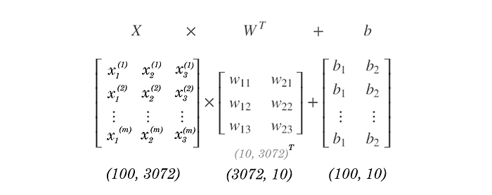
Following along with the matrix multiplication, we get a (100, 10) matrix with each row being a training example, and each column being some scalar value associated with the probability that training example is each label.
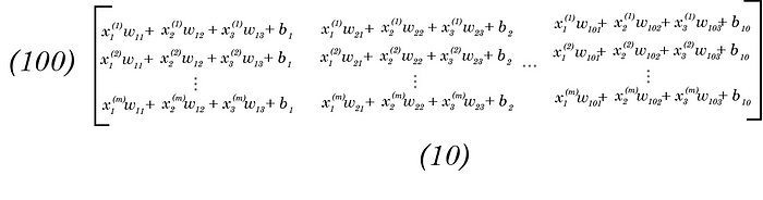
Therefore, the predicted “probabilities” for each class for one training example is each row. I put probabilities in apostrophes since these aren’t classical 0–1 probabilities, but scalar numbers of any size (they are just the products of a linear expression). Softmax converts these to probabilities, which we’ll go over soon.
>> import torch.nn as nn# this will dictate the rows of the weights matrix>> inputSize = 3*32*32# this will dictate the columns of the weights matrix>> numClasses = 10# create our linear regression model (nn.Linear creates bias terms for us)>> model = nn.Linear(inputSize, numClasses)
nn.Linear creates the weights and biases, creating a matrix of shape (imputSize, numClasses). More than just that, nn.Linear creates a function model, which can later be passed a matrix of training examples in order to return predictions. Additionally, nn.Linear also randomly initializes the values of each weight and bias.
Essentially, nn.Linear creates the bias and weights matrix automatically given the amount of classes and amount of features. When we pass something into the model created by nn.Linear, we are just multiplying by the weights matrix and adding the bias.
>> print(model.weight)Taking a sneak peak at our weights, we can see they are all miniscule values such as -1.0100e-02, all with requires_grad = True. requires_grad = True means that PyTorch allows these values to be differentiated, once we get to gradient descent (the reason why this is an option is that computing derivatives is costly, so PyTorch makes sure to only do this when it is absolutely necessary).
But, if we try to fit our training examples (trainLoader) to this model, we get an error. This is because trainLoader is a matrix of shape (100, 3, 32, 32), which cannot be multiplied by our weights matrix in nn.Linear which is of size (3072, 10).
Matrices can be multiplied if the first matrix’s columns is the same as the second matrix’s rows. So, we need to find a way to turn trainLoader (100, 3, 32, 32) into something compatible with (3072, 10).
The obvious choice would be to reshape trainLoader into size (100, 3072), but let’s instead edit the class nn.Linear itself to change the function to automatically reshape any trainLoader, regardless of size, into a compatible matrix. This can be done with Python classes.
>> class CIFAR10(nn.module):
      def __init__(self):
        super().__init__()
        self.linear = nn.Linear(inputSize, numClasses)
      def forward(self, xb):
        xb = xb.reshape(-1, 3072)
        out = self.linear(xb)
        return out>> model = CIFAR10()
What this code does it creates the CIFAR10 class, which builds off the nn.Module class (and thus gains all of it’s methods and functions).
It creates itself using def __init__. Then it defines a new function, forward(self, xb) where xb is a batch of training examples (x-batch).
Forward automatically reshapes the training examples into shape (-1, 3072). Using -1 means that the new matrix will have however many rows it needs to have 3072 columns. Since our original xb (100, 3, 32, 32) would have a total of 307200 items (100 x 3 x 32 x 32), the -1 solves for what amount of rows would hold the same amount of items. (solving for x in 3072x = 307200).
The reason why we do this, and don’t hardcode (100, 3072), is that it adapts to different batch sizes.
Then we set the output of the function as our new xb through the same nn.linear function.
the .forward() function of a model is assumed when we do Model(xb) — there is no need to specify Model.forward(xb). That’s to say, by creating our own class CIFAR10, and redefining the definition of forward, after setting our model to an object of class CIFAR10, to CIFAR10(xb) will fit the model.
Since model = CIFAR10, we now just need to execute model(dataLoader), and not model.forward(dataLoader), to get the program to work, since forward now automatically reshapes the values.
>> print(model.linear.weight.shape)
>> print(model.linear.bias.shape)
We can still check the parameters of our model, even though we modified the overarching class. Since CIFAR10 is a subclass of nn.Module, it gained all of nn.Module’s methods, like model.linear.
Using these codes, we can still check the shapes of the weight and bias matrices.
Now we can finally get our initial predictions, by passing trainLoader into our modified model. Remember, ‘passing trainLoader in our model’ is equivalent to multiplying our training values by our paramaters and adding a bias, just done in a built in function.
>> for images, labels in trainLoader:
     outputs = model(images)
     break>> print('outputs.shape :', outputs.shape)
outputs.shape : torch.Size([100, 10])
A for loop over trainLoader iterates over the batches. Since we use break in the for loop, we only calculate the initial predictions for the first batch in trainLoader.
Checking the shape of outputs gives a matrix of (100, 10), which matches our initial calculations. There are 100 rows, for each example (image) in the batch, and each of the 10 columns contain the probability that the image (row) is in each class (horse, sheep, etc..). Only one problem — these probabilities are logits, arbitrary real numbers calculated by the model.
Why? When we multiply our inputs by some random weights and adding a bias, nothing’s restricting it to be a probability — they’ll all be random products, like 3.21324, and not probabilities that are between 0 and 1 and add up to 1.
But first, let’s recap. What have we done so far?
1. Import dataset and transform images to RGB matrices of 3x32x32.
2. Split dataset randomly into 50000 training examples and 10000 validation
3. Via SubsetRandomSampler, the dataset is shuffled once again into an iterative object.
4. Via DataLoader, the randomly shuffled indexes paired with corresponding image matrices, in preset batches decided by batchSize.
5. Modify the nn.linear function by editing the class nn.model, and making it so that nn.linear automatically flattens a matrix before entering it in nn.linear
6. Inputting the number of classes (X’s rows) and number of features (X’s columns) into nn.linear gives us a model, and empty set of weights to multiply something by.
7. By iterating through our trainLoader, which contains both the image matrix and the labels, we can input the image matrices through our model to get our outputs.
Let’s print out the predictions for the first two examples.
>> print('sample outputs :\n', outputs[:2])
sample outputs :  tensor([[-0.2363,  0.4695, -0.0422, -0.3637, -0.0558, -0.2168, -0.0343, -0.0593, -0.2294,  0.8198], [-0.2203,  0.1576,  0.4396, -0.2661, -0.2340, -0.2024,  0.2856,  0.1390, -0.6146,  0.6665]], grad_fn=<SliceBackward>)
Each of the two images have 10 probabilities, which stand for the probabilities each image has for belonging to any of the ten classes.
The numbers seem random (and indeed they are, they’re simply the linear product of the weights and the bias, without any nonlinear function like sigmoid attached).
This is where we need the softmax function.
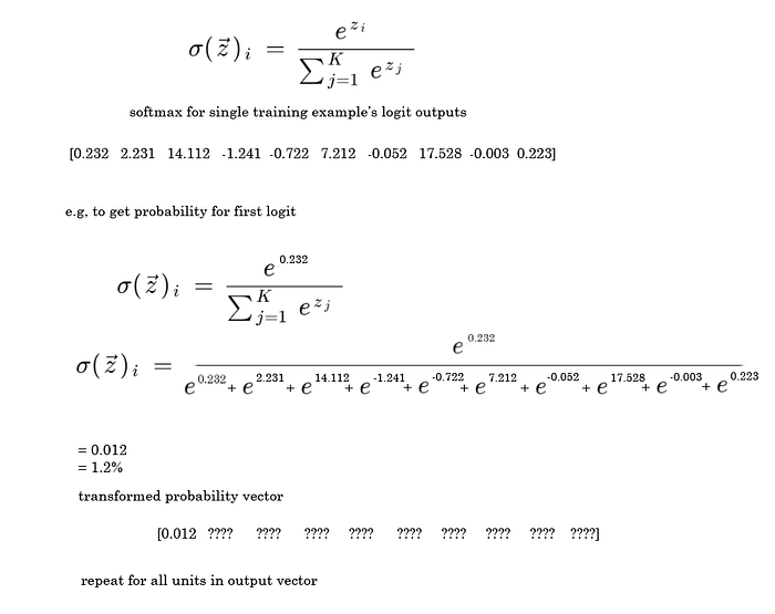
The softmax function
The numbers that outputs contains are called logits. Here, we can understand logits to be numbers that represent probabilities, but not in the classical sense of adding up to 1. They represent some amount of likelihood, but not concretely. The larger a number is, the larger the probability. How do we convert these logits into standard probabilities (between 0 and 1) that also add into one?
I stole this fantastic explanation from Ritvik Kharkar’s youtube channel, ritvikmath, so check that video out.
How would we turn one training example’s logit row vector into an equally sized row vector of probabilities?
So, why do we need the exponentiation (e’s) in the numerator or denominator? Why not just add up each unit of the outputs vector divided by the sum, and rid of the exponentials?
Well, say if we did do this.

There’s one problem with not using exponentiation. If we add some constant to all of our terms, our probabilities change significantly. This shouldn’t be true — our probabilities should be calculated on how they big they are relative to each other.
Exponentiation solves this problem.

All in all, softmax is a wonderful, and strikingly intuitive way to compress logits into probabilities.
We can implement this in Pytorch quite easily:
>> import torch.nn.functional as F# apply the softmax for each output row in our 100 x 10 output (with batch size 100). Specifying dim=1 makes softmax work horizontally, which is correct since the columns are what we want to softmax over>> probs = F.softmax(outputs, dim=1)
We can now check to see if our logits have been converted into probabilities:
# look at some sample probabilities>> print("sample probabilities:\n", probs[:2].data)sample probabilities:
tensor([[0.0733, 0.1485, 0.0890, 0.0646, 0.0878, 0.0748, 0.0897, 0.0875, 0.0738, 0.2108],

[0.0738, 0.1077, 0.1428, 0.0705, 0.0728, 0.0752, 0.1224, 0.1057, 0.0498, 0.1792]])
And indeed they have. Sanity checking each row to see if they add up to one will return 1 or a number very close, like 0.99992282, due to floating point error (basically, rounding issues).
Our prediction, then, is the largest probability for each training example, which can be found by finding the maximum across each row (dim=1) using torch.max.
# torch.max returns the max value itself (maxProbs) as well as the index of the prediction (preds). Since our labels are from 0-9, the indexes of the maximum is the class the predictor predicts.>> maxProbs, preds = torch.max(probs, dim=1)
We can then print our predictions (preds) to see what our randomly initialized model predicted for our first batch.
>> print(preds)
tensor([9, 9, 9, 9, 6, 9, 9, 9, 9, 9, 9, 1, 9, 9, 9, 9, 9, 9, 9, 6, 9, 9, 9, 9, 1, 9, 9, 9, 9, 9, 9, 9, 9, 9, 9, 9, 9, 9, 9, 9, 9, 9, 9, 1, 9, 9, 9, 9, 9, 9, 9, 9, 9, 9, 9, 9, 9, 1, 9, 9, 9, 9, 1, 9, 2, 9, 9, 9, 9, 9, 9, 9, 9, 9, 9, 9, 9, 9, 9, 9, 9, 9, 9, 9, 9, 9, 9, 9, 9, 9, 9, 9, 9, 9, 6, 9, 9, 9, 9, 9])
It looks as though, with randomly initialized parameters, our images seem to be predicted as 9 (truck) quite often. Ponder why that may be.
evaluation and accuracy
A natural way to evaluate the accuracy of the algorithm is by seeing when our predictions match the labels given, or, when labels == preds (which returns a boolean array of when our predictions matched the ‘right answer’.
>> labels==predstensor([False, False, False, False, False, False, False, False, False, True, False, False, False, False, False, False, False, True, False, True, False, False, False, False, False, False, False, False, False, False, False, False, False, False, True, False, False, False, False, False, False, False, False, False, False, False, True, False, False, False, False, False, False, False, False, False, False, False, False, False, False, False, False, False, False, False, False, False, False, False, False, False, False, False, False, True, False, False, False, False, False, False, False, False, False, False, False, False, False, False, False, False, False, False, False, True, False, False, False, False])
Now, we can create a function that adds up all the trues and divides by the total to get our accuracy percentage.
>> def accuracy(preds, labels):
      # this works since True = 1 False = 0
      return torch.sum(labels==preds).item() / len(labels)
And…
>> accuracy(preds, labels)0.07
But this isn’t a good cost function at all.
Since during gradient descent, we calculate the derivatives of the cost function w.r.t every parameter, the cost function must be continuous and differentiable. How do you differentiate max()? How do you differentiate ‘==”? It’s impossible.
Additionally, although accuracy can give a good, understandable, evaluation metric, it doesn’t reflect minute changes in predictions — an algorithm that predicts 0.2 for the correct answer is better than one which predicts 0.1, but the accuracy could still say ‘False’ — how would the algorithm improve?
That’s where our cross entropy loss comes in.
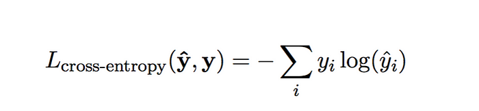
categorical cross-entropy cost function
We must first describe each right answer (yhat) as a vector (as opposed to a scalar, like 7), using one-hot encoding. For example, the one-hot version of the right answer being 3, 0 and 8 respectively would be:
[0 0 0 1 0 0 0 0 0 0 ], [1 0 0 0 0 0 0 0 0 0 ], [0 0 0 0 0 0 0 0 1 0 ]
We then take this, and multiply it by taking the elementwise natural logarithm of our predicted values.
Here’s a walkthrough for a single training example if the right answer was 3.
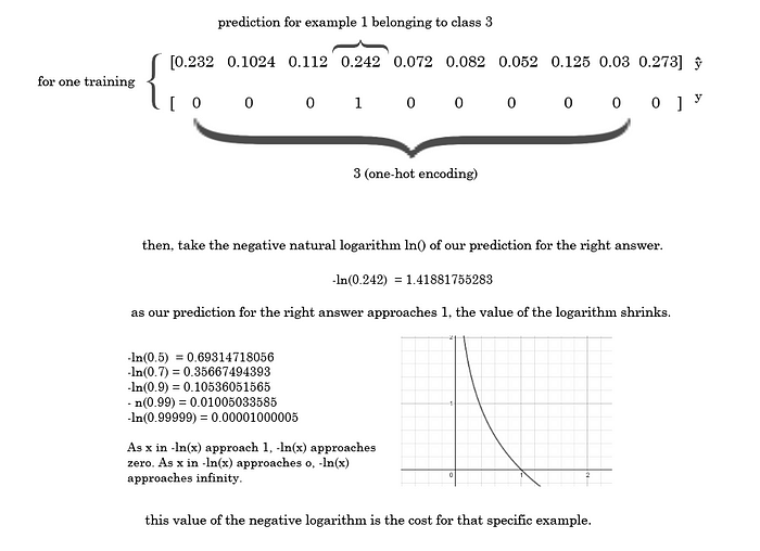
By multiplying the natural logarithm of the entire predictions vector by the one-hot encoded vector, we can effectively eliminate the cost except for the right answer, because everything else would be multiplying by zero.

After dotting the one-hot y vector and the predicted probability yhat vector, we are just left with 1 times the -ln() of the probability our model predicted for the right answer. This quantity is the cost for the example.
The Categorical Cross-Entropy Function is a good choice for our cost function since it is differentiable and continuous.
Most implementations of categorical cross entropy take the average of the sum for each batch to calculate the average loss for that batch. Then, the averages on the batch are averaged over all batches for a final, single scalar value.
Additionally, some small improvement in percentage for one example will improve the overall cost, as we are dealing with the continuous prediction percentages and not the discrete “Right/Wrong” that the accuracy evaluation gives.
>> import torch.nn.functional as F>> lossFn = F.cross_entropy# loss for current batch of data >> loss = lossFn(outputs, labels)
tensor(2.3579, grad_fn=<NllLossBackward>)
In PyTorch, cross_entropy computes softmax automatically, so the outputs that we pass in are the raw (100, 10) matrix outputted by our model, with logits instead of probabilities. Our labels are the (1, 100) right answers row vector.
mini-batch gradient descent
The problem with batch (standard) gradient descent is that it can very quickly become slow when computing with large datasets and or large amounts of features.
This is because on each iteration (an epoch) of gradient descent, the derivatives w.r.t all of the weights and biases have to be calculated (to form the gradient) as well as summing over the entire training set. When we get into the millions of training examples, or even with our m =50,000 and n (number of features) = 3072 + biases, this can get computationally expensive fast.
Thus, we need a smarter, quicker way to execute gradient descent.
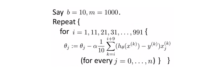
Mini-batch gradient descent involves splicing your training set (both your X’s and your labels) into batches of some specific size (usually from 50–256). Recall we did this earlier on in our code by using SubsetRandomSampler and DataLoader with predefined batch size of 100.
Then, looping over our DataLoader (split into batches of 100, where each iteration over DataLoader accesses a new batch), we can calculate the gradient w.r.t all parameters for a smaller subset of 100 examples.
Then, we can take a step (change all parameters slightly) based on the gradient calculated with the batch of 100 — an approximation, if you may, of the actual gradient of the entire dataset.
We can then do this for all batches in the dataset. So, in a scenario where you had 450 batches, you would take 450 steps of gradient descent based on the gradients calculated from each batch. Despite this, you to complete a true ‘iteration’ or epoch of gradient descent, you must run through all 450 batches. Only once you start reusing batches are you onto your second epoch.
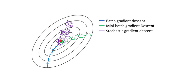
First, a quick clarification — mini-batch gradient descent is quite different form stochastic-gradient descent but the terms are sometimes used interchangeably. Stochastic gradient descent is essentially mini-batch gradient descent with batch size of one. If batch sizes larger than one are discussed, we are dealing with mini-batch and not stochastic — this is important to note as a lot of code misleadingly refers to mini-batch as ‘stochastic’ — we see an example of this in the code below (SGD = stochastic gradient descent)
learningRate = 0.001
optimizer = torch.optim.SGD(model.parameters(), lr=learningRate)
This code tells us to improve the .parameters() of our model using mini-batch gradient descent, and a learning rate of 0.001.
If you want the mathematical derivations of both this and softmax, those will be at the bottom of the article.
training the model
computing derivatives for single batch
Now that we have our loaded data, model, cost function and optimizer, we can begin fitting and training our model.
# recall that xb is the X (a list batchSize long of 3x32x32 images) for a batch. yb is the corresponding labels for those images.>> def lossBatch(model, lossFn, xb, yb, opt=None, metric=None):
   # calculate the loss
   preds = model(xb)
   loss = lossFn(preds, yb)   if opt is not None:
       # compute gradients
       loss.backward()

       # update parameters
       opt.step()

       # reset gradients to 0
       opt.zero_grad()metricResult = None
if metric is not None:
   metricResult = metric(preds, yb)return loss.item(), len(xb),  metricResult
The code above defines a function that calculates the loss, then derivatives w.r.t the parameters for a single batch(xb, yb) with [mini-batch] gradient descent.
It also optionally computes a metric of some sort, for example, accuracy, which isn’t a cost function but a good benchmark for evaluation.
This code then returns the loss of that specific batch, the length of that batch, and the result of the metric from that batch.
Note: an optimizer is an optional input since we want the lossBatch function to work in another context, without optimization, as we’ll see shortly.
Evaluating cost and accuracy on validation set
To properly monitor progress in training, we want to view the cost and accuracy from our validation set as opposed to our training set, to avoid any possible overfitting errors.
>> def evaluate(model, lossFn, validDL, metric=None):
    with torch.no_grad      # why we made optimization optional on lossBatch      results = [lossBatch(model, lossFn, xb, yb, metric=metric) for
      xb,yb in validDL]     # separate losses, counts and metrics from multidim. list
      losses, nums, metrics = zip(*results)     # total size of the dataset
      total = np.sum(nums)     # find average loss over all batches in validation
      avgLoss = np.sum(np.multiply(losses, nums))/total     # if there is a metric passed, compute the average metric     if metric is not None:
       # avg of metric accross batches
       avgMetric = np.sum(np.multiply(metrics, nums)) / totalreturn avgLoss, total, avgMetric
We use the same lossBatch function, sans the optimization, to get the loss, length, and metric evaluation on each batch in the validation set.
We then use a list comprehension to create a multidimensional list containing the losses, lengths and metrics for each batch, which we can then unzip into three different lists.
The reason we keep track of the length of each batch, instead of just multiplying batchSize, is that our dataset might not be perfectly divisible by batchSize, leading to incorrect averaging.
We can then compute the average loss, and if a metric is passed, the average evaluation metric.
The function returns the average loss, total size, and average evaluation metric number for the entire cross-validation set, based on the model inputted.
Redefining the accuracy metric
Before fitting the final model, we must first redefine our accuracy metric to directly deal with the raw outputs (product of weights and X + bias) for each batch (a 100 x 10 matrix of logits).
>> def accuracy(outputs, labels):
     _, preds = torch.max(outputs, dim=1)
     return torch.sum(preds == labels).item() / len(preds)
Since the largest logit in a row vector of probabilities for one example will still be the largest probability when converted to probabilities via softmax, we can directly take index of the maximum of the logits as our prediction for each training example. Keep dimensions to 1 to compute across columns.
Now, our predictions is a vector of 100 numbers from 0 to 9, which is of analogous type to our predictions for that batch, we can create a boolean vector and sum over the correct predictions and divide by the total to get our accuracy.
sanity checking
We can check our preliminary losses on the cross validation and training sets with our randomly generated weights. The loss should be quite similar.
>> Etrain = evaluate(model, lossFn, trainLoader, metric=accuracy)
>> Eval = evaluate(model, lossFn, valLoader, metric=accuracy)>> print("training set loss: ", Etrain[0])
 2.3579
>> print("cross validation set loss: ", Eval[0])
 2.3416
If they aren’t, that means there is likely something wrong with the organization of either your training or cross validation sets.
fitting the model
Finally, we can iterate through our desired epochs and improve our model.
>> def fit(epochs, model, lossFn, opt, trainDL,
   valDL, metric=None):
       valList = [0.10]       for epoch in range(epochs):          # training - perform one step gradient descent on each
          batch, for all batches          for xb, yb in trainDL:
            loss,_,lossMetric=lossBatch(model, lossFn, xb, yb, opt)          # evaluation on cross val dataset - after updating over
          all batches, technically one epoch          # evaluates over all validation batches and then
          calculates average val loss, as well as accuracy          valResult = evaluate(model, lossFn, valDL, metric)
          valLoss, _, valMetric = valResult           valList.append(valMetric)          # print progress          if metric is None:
             print('Epoch [{}/{}], Loss: {:.4f}'.format(epoch + 1
                   epochs, valLoss))          else:
             print('Epoch [{}/{}], Loss: {:.4f}, {}:
             {:.4f}'.format(epoch + 1, epochs, valLoss,
             metric.__name__, valMetric))return valList
First, we initialize a list that will update with the new cross validation accuracy upon each epoch. We enter a placeholder ‘untrained’ accuracy, around 0.10, which is the accuracy of the model before gradient descent.
Then, we start a for loop around the amount of epochs inputted.
First, upon each epoch, mini-batch gradient descent is carried out on all batches in the dataset. Once we step the algorithm using lossBatch, we then evaluate the new model on the cross validation set using our predefined evaluate() function, which records the accuracy and loss on validation.
We append the validation accuracy to our list.
Then, we print our progress at the end of the epoch — our current loss, and if a metric was passed, current accuracy. Since this is printed every epoch, it will be a helpful way to view how the model has improved.
Let’s now finally implement all the code we wrote. First, redefine some of the outputs, as well as the model.
# redefine model and optimizer
>> learningRate = 0.003
>> model = CIFAR10()
>> optimizer = torch.optim.SGD(model.parameters(), lr=learningRate)
Then, we can execute fit() to see our model improve.
>> trainList = fit(100, model, lossFn, optimizer, trainLoader, >> >> valLoader, metric=accuracy)The output, for the first ten epochs, should look something like this.
Epoch [1/100], Loss: 2.0002, accuracy: 0.3011
Epoch [2/100], Loss: 1.9263, accuracy: 0.3366
Epoch [3/100], Loss: 1.8895, accuracy: 0.3525
Epoch [4/100], Loss: 1.8611, accuracy: 0.3630
Epoch [5/100], Loss: 1.8486, accuracy: 0.3650
Epoch [6/100], Loss: 1.8401, accuracy: 0.3684
Epoch [7/100], Loss: 1.8340, accuracy: 0.3675
Epoch [8/100], Loss: 1.8189, accuracy: 0.3757
Epoch [9/100], Loss: 1.8143, accuracy: 0.3735
Epoch [10/100], Loss: 1.8058, accuracy: 0.3779
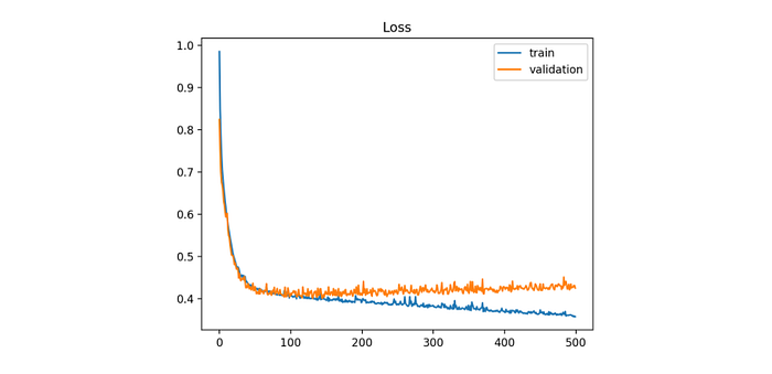
....Since our fit() function returns a list of the validation accuracies for each epoch, we can use matplotlib.pyplot to plot these as a function of epochs to visualize how our weights and biases are improving.
plt.plot(trainList, '-x')
axes = plt.gca() #gca means get current axes
axes.set_ylim([0,1])
plt.xlabel('epoch')
plt.ylabel('accuracy')
plt.title('accuracy vs number of epochs')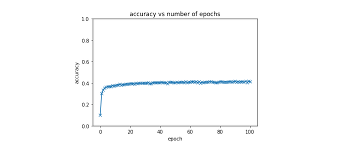
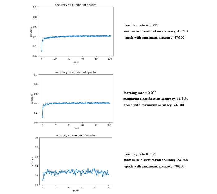
Playing around with the learning rate for this model, I found the best to be at 0.009, where the maximum classification accuracy I was able to achieve was 41.71%. Here are three examples with different learning rates:
What our algorithm does
1. Downloaded our data from torch.datasets
2. Transformed them into tensors of pixel color values in shape (3, 32, 32)
3. Split into training and validation sets
4. Loaded into batches of 100 using SubsetRandomSampler and DataLoader
5. Load batches into model
6. For every epoch, calculate gradient descent on all batches (mini-batch gradient descent)
7. Using parameters calculated in gradient descent, evaluate these and get cost and accuracy on the validation set.
8. Repeat step 6 and 7 for every epoch.
Is low accuracy inevitable with logistic regression?
Knowing that our algorithm peaks in accuracy at around 41–42%, with a learning rate of around 0.009 is low accuracy inevitable, or a product of error within the code?
Obviously, training has worked somewhat, as we’re considerably higher than the untrained classification accuracy which floats around 10%.
Nonlinearity of outputs
Logistic regression is a linear function because the predicted outcome is always a sum of the parameters and not a product of them (never w1·w2, only w1 · x1) Logistic regression works best when predicting linear (directly correlated) relationships between the inputs and outputs. It is similar to linear regression in that way.
A linear relationship is one that can be expressed by an infinitely long, straight line between the independent and dependent variables. An example would be that a temperature of 25° outside would increase profit from a lemonade stand by 15%. If the temperature increased to 130°, a linear relationship would predict some seriously high profit, even if it means everyone is dead.
A nonlinear relationship would identify that there is a point, where heat gets so extreme that profits begin to drop again.
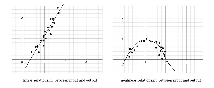
The patterns within an image, especially those from more complex datasets like CIFAR-10 (as opposed to something like MNIST), cannot be properly modeled by linear relationships.
Additionally, with ten classes, there is less of an obvious difference from class to class in terms of color values present in each pixel, as there are more ‘niches’ filled, which makes nonlinear functions even more integral to accurate classification.
Concretely, imagine that we had one pixel. Looking at this pixel’s specific green and blue channel, we would be viewing 2 out of the 3072 features in our dataset. If we were to plot the values of these channels from 0 to 256, we could see that with 10 classes, it would be impossible to separate them all accurately with a linear decision boundary.
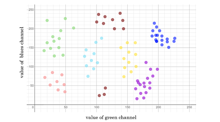
It’s a bit challenging to think about, but finding how to encircle (using the decision boundary) each group of coordinates for blue/green values of a pixel is equivalent to finding the best weights. To determine which class a new example belongs to is tough without nonlinearity.
Code
Here’s the full chunk of code (on Google Colab) I’ve been referencing to pieces throughout this assignment. It’s what I did from following this fantastic tutorial, but applying the principles to a slightly different dataset.
Thanks for taking the time to following along this monstrously long tutorial, or even if you stopped by just for some parts.
Lookout soon for a similar tutorial on using neural networks on CIFAR-10 and seeing how that affects accuracy. After that, I’ll be writing the last article in this miniseries, which will be using a convolutional neural network.
Deriving the update rule for parameters
This is a bit more disjointed from the rest of this tutorial, so here’s the update rules as an optional second part to this tutorial — warning, it requires a pretty good understanding of calculus and neural network backpropagation.
Adam Dhalla is a high school student out of Vancouver, British Columbia, currently in the STEM and business fellowship TKS. He is fascinated with the outdoor world, and is currently learning about emerging technologies for an environmental purpose. To keep up,
Follow his Instagram , and his LinkedIn. For more, similar content, subscribe to his newsletter here.