Thinking about logistic regression as a simple neural network gives an easier way to determine derivatives.

Gradient Descent Update rule for Multiclass Logistic Regression

Deriving the softmax function, and cross-entropy loss, to get the general update rule for multiclass logistic regression.

This is continuing off of my Logistic Regression on CIFAR-10 article, so skim that for some details —especially the intuition on cross-entropy and softmax.

Complete Guide: Image classification on CIFAR 10 chapter I : Multiclass Logistic regression

Here are a few details about the CIFAR-10 image dataset this article is being written in the context of.

• CIFAR-10 has ten possible classes.
• CIFAR-10 has 3072 features per example (color pixel values in an image)

I’d recommend a good knowledge of derivatives and simple neural network functions, like backpropagation for this part. Even if you do know those things, you won’t understand just from reading this. Work through the problem yourself, and solve the problems you encounter.

A second disclaimer — out of simplicity, all of this will be assuming a single training example.

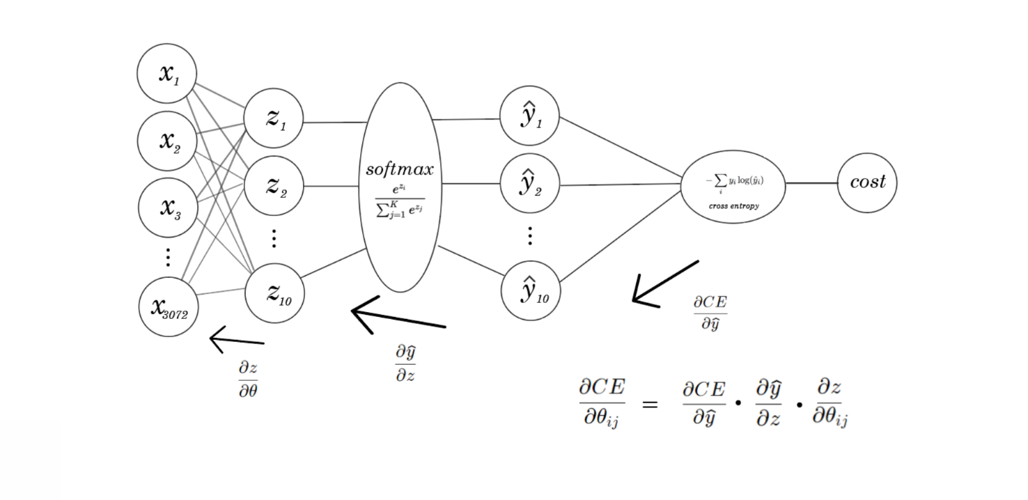
To derive the update rules of the parameters, it helps to think of logistic regression as a simple neural network, with zero hidden layers.

Much of this proof is from this fantastic lecture:

If you’re familiar with the computation of a neural network, this will make quite a bit of sense. I’ve omitted bias terms as they don’t really add anything intuition-wise.

The update rules for each parameter is the partial derivative of the loss function w.r.t the parameter in question.

Our update rule is still the same as linear regression, except that instead of finding the derivative of the least squares cost function, it’s the cross entropy function.

Where the weights matrix has training example weights as rows and classes as columns.

With linear regression, we could directly calculate the derivatives of the cost function w.r.t the weights. Now, there’s a softmax function in between the θ^t X portion, so we must do something backpropagation-esque — use the chain rule to get the partial derivatives of the cost function w.r.t weights.

We can use chain rule to ‘backpropagate’ through our logistic regression model.

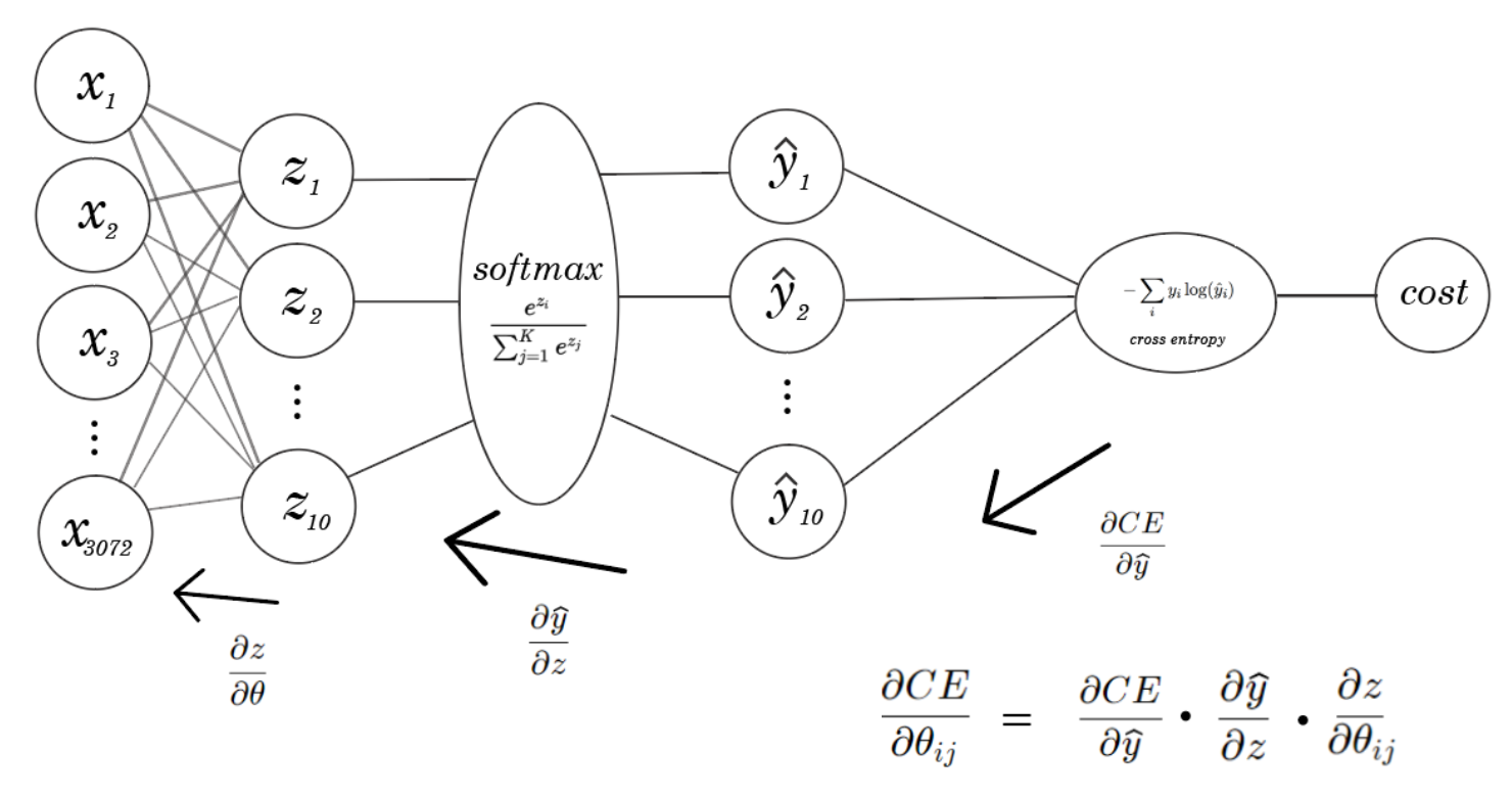
So, we’ll need to find the derivatives of the loss function and the softmax function.

Deriving the softmax function

The biggest thing to realize about the softmax function is that there are two different derivatives based on what index of z and y you’re taking the derivative from. Don’t necessarily think of Z and Y as vectors, but as 10 individual numbers that are passed element-wise through the function.

Remembering that K is the amount of classes, i the class you want to find the probability of, and j, what indexes through the classes.

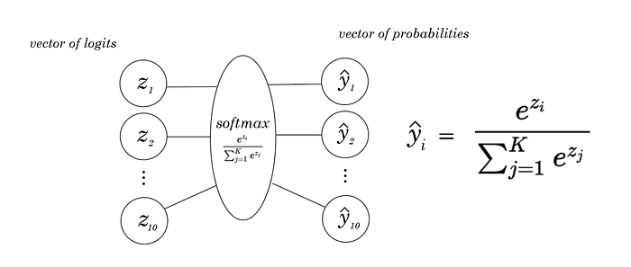
If you haven’t noticed, the softmax is a function of not just the zi that it is linked to, but the entire ‘layer’ of z’s before it, since the denominator of the softmax sums over all logits in the training example.

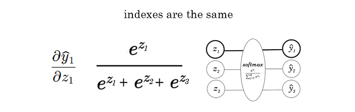
Concretely, with a simpler example — with only three inputs.

The important thing to note is the values of the output yhats.

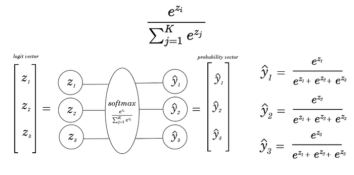
Notice that all the output y’s are functions that have all z’s from the layer before as outputs — specifically, in the denominator. Thus, there are two ways to take the derivative.

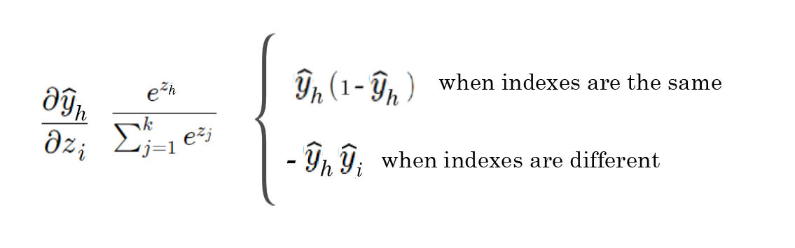
Where the y index and z index match: for example, find the derivative of the first yhat in our example with respect to the first z1.

Where the y index and z index don’t match, for example, taking the derivative of yhat1 with respect to z2.

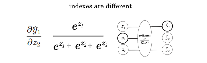
These two cases return different derivatives, as you’re essentially taking the partial derivative of the same thing with respect to a different variable. Let’s derive both ways, starting with when the indexes are the same.

Here, we use h to signify the index of yhat, and i to signify the index of z.

And, now when they’re different.

So once we’re done, we end up with two different derivatives for different scenarios of the softmax function.

Now, how do these play in the derivative of cross-entropy loss?

Deriving categorical cross-entropy loss

Our goal is to find the derivative of the cost function with respect to the weights of the model.

j subscript here unrelated to our usual use of j as an indexing subscript

But once we have z, it’s easy to calculate the derivative w.r.t theta, since it’s a simple linear function (z = θTx +b, differentiate w.r.t θ), so, for the sake of simplicity, let’s temporarily try to find the derivative of the cost function with respect to z.

The i means that we need to find a derivation of the cost function that works for any z.

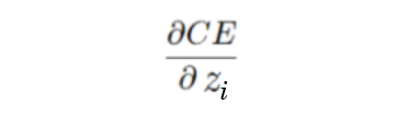
Since we already have our loss function, let’s just take the derivative of this w.r.t z and see where it goes. Remember again that whenever I’m using log() it means ln().

Remember that h is the index of yhat, and i is the index of z.

Also, I forgot to put limits on the summations, but they go on for however as many classes exist.

Now, using both of the softmax derivatives we derived in the previous section, let’s derive the cost w.r.t some arbitrary zi term.

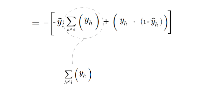
Remember that the summation in the cross entropy derivative sums over i, or each class in the training set. Recall that we have two different versions of the derivative for the softmax function.

So, we can drag the i = h term out of the summation (since there is only one occurrence of this in each training example). We can then sum over the main i does not equal h loop, and only exit it to compute the one instance per training example where i is = to h.

A concrete example helps a lot.

Say we had three classes and wanted to find the derivative of the cost with respect to z2: so, our i = 2 .

Now that we know how this works, all we have left to do is simplify our new derivative of the loss function with respect to z.

We can clean this up further by exploiting the fact that we are using one-hot encoded vectors. One hot encoded vectors have the following property that:

where c is the amount of classes in each training example.

If we are summing over the elements of the one hot vectors, the sum should be 1 no matter what, since our vector contains just zeros and one one.

Is there a way we can simplify this summation in our derivative of cross entropy using similar logic? We are still summing over the one-hot vector, after all — just without the value in the vector that matches that of h.

Well, sure. We can express this summation as the summation of the total y vector minus the ysubi value — now they’re equal.

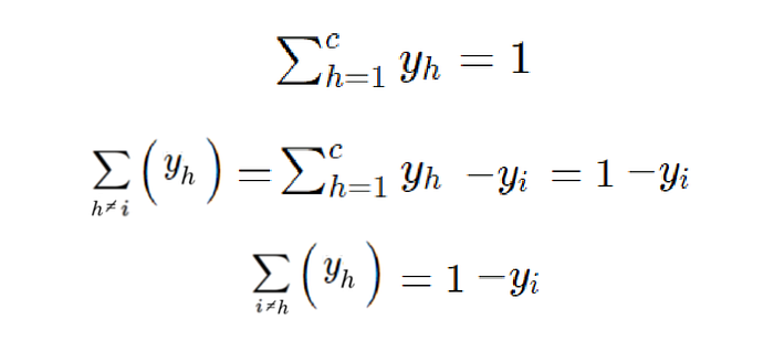
Now, we can replace that definition within our derivative.

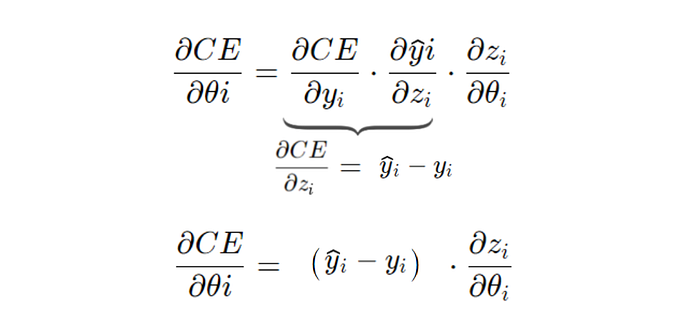
Isn’t that the most satisfying feeling in the whole world? That entire function’s derivative boils down to just two terms, the predicted y minus the actual y.

It’s almost how magical the derivative turns out to be so simple.

This final derivative is the derivative of the cost function w.r.t any individual z — since we took into account both versions of the softmax’s derivative.

To revist our old example, where we find the derivative of the cost function w.r.t z2, let’s actually calculate that now.

A little too easy, huh.

Deriving update rules for weights in gradient descent

Now, we can easily find the update rule with respect to each of the weights by finding the derivative of z with respect to the weights.

Now we just need to find how z changes w.r.t theta.

Let’s continue to think about this with one training example.

This would be the calculation for one training example. Note the indices on the theta matrix — something like 101 means class 10 weight 1

If we write out the actual calculations for this vector-matrix product (or, the value of each z), we get something like this:

This will be clearer by doing the multiplication above.

We can express each z as a sum of products — to find a general update rule for all the weights (thetas), we can take the derivatives of these sums.

For example, if we’re just focusing on z1, we can express this sum with sigma notation, and derive this.

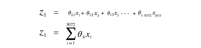
We can now take a derivative of z1 w.r.t to θ1i, which would give us the general update rule for all theta’s for class 1 (or the first column of the theta vector).

Getting rid of the summation can be a bit confusing, so consider this thought experiment:

Imagine a summation that goes from 1 to three, with θ1, θ2, and θ3 and x1, x2, and x3. Say we wanted to take the derivative of the summation with respect to θ2.

We can expand this logic towards a more general problem like our own — all the other elements in the summation would be eliminated since you’re they’re affiliated with some i-1 or i+1, but not i.

We can now expand our derivation to any class — let’s take the derivative of z2.

We can see that our update rules are independent of our class — despite the class we’re dealing with, the derivative is just the feature x which the theta we are updating is multiplying by — for example, if we’re dealing with θ2 1032, the derivative would be x1032 — unrelated to the class of 2.

Now that we have a general derivative for z (xi) w.r.t to any weight, we can replace this in our grand chain rule operation for the update rule.

Now that we have this, we can substitute it in our general gradient descent update rule.

All that work for our update rule.

That’s it. That’s how every weight is updated.

Adam Dhalla is a high school student out of Vancouver, British Columbia, currently in the STEM and business fellowship TKS. He is fascinated with the outdoor world, and is currently learning about emerging technologies for an environmental purpose. To keep up,

Follow his Instagram , and his LinkedIn. For more, similar content, subscribe to his newsletter here.